
Dynamics of LMP Pricing
Ted Leffler is a senior economist at Indianapolis Power & Light Company (IPL), an AES Company. He is an expert in wholesale power-related issues.
Bob Shively is President of Enerdynamics Corp., which partners with energy companies to provide education programs. He is an expert on competitive energy markets and implementation of new energy technologies.
As renewables are increasingly added to the grid, market participants are finding that energy revenues from both new and existing generators may vary significantly from their expectations. As policymakers consider subsidies for other types of generation such as nuclear or other baseload units and corporations invest in grid scale renewables, understanding price formation becomes increasingly important.

Transmission expansion can change revenues for the better or worse too. Meanwhile, loads also experience unexpected effects as energy costs in a specific region vary significantly from forecasts that were based on historic price behavior.
Comprehending how new units, generation subsidies, and transmission expansion impact energy revenues is predicated on understanding how Independent Transmission System Operators (ISOs) determine which units run, the levels at which they run, and the market prices at which they run. The methods employed by ISOs are quite complex, and it can be difficult to forecast expected outcomes.
This article provides a simple two-region model that demonstrates how ISOs make such decisions. By doing so, the model provides high-level insights that can be used to help policy makers, regulators, investors, market participants, and other interested parties see many of the controversial and complex industry issues.
Results that can be observed include extreme locational and time-based energy market price differences, including low or even negative prices and disparities in generation revenues and load costs that reward some market participants and penalize others. Those disparities are based on location and non-intuitive dispatch decisions that may result in displacement of nuclear or gas units while coal units continue to run. We also observe that expanding transmission can sometimes be more effective in reducing greenhouse gas emissions than adding more renewable generation.
 Bob Shively: In a perfect world, the transmission system would be robust enough to allow the ISO to dispatch this optimum set of resources.
We will first describe the two-region model, then walk through various examples.
A Two-Region Model
The model consists of a Left and Right Region, connected by one transmission line (Path A) which transfers energy from the left to the right. Four 200-megawatt generating units reside in the Left Region, and four in the Right Region, each offering 200 megawatts into the ISO energy market at each unit's variable cost.
One load-serving entity resides in each region, and the transmission grid in each region has enough transmission to deliver its electricity to the load within that region. Transmission between the regions may be constrained, depending on operating conditions.
The Left Region could represent a rural area near coal reserves, resulting in lower variable cost, with the Right Region representing an urban area in the same state with higher variable costs. Alternatively, the Left Region could be in a wind generation center (such as Iowa or North Dakota) and the Right Region could be a densely-populated region without the space for utility scale wind units (such as Chicago).
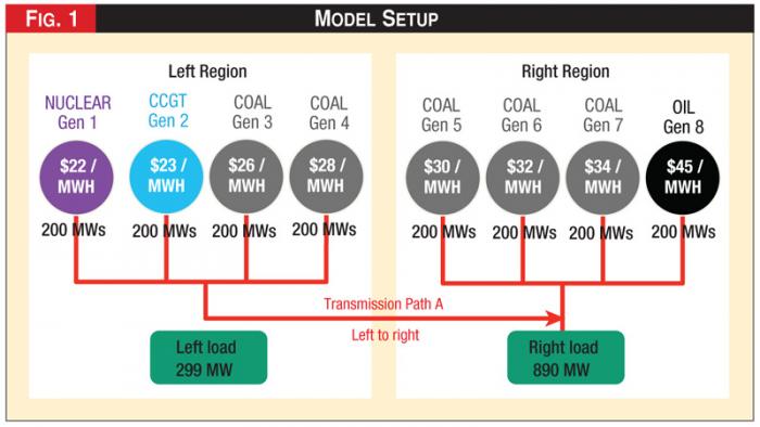 Figure 1 - Model Setup
See Model Setup.
Dispatch Outcomes Under Various System Conditions
We will now look at price outcomes in the two regions under various conditions. To simplify the discussion, we will only look at day-ahead prices for a single hour. We will ignore the impact of transmission losses and generation operational limitations.
To maintain system balance, the ISO selects a set of resources that will generate megawatts equal to total system load requested by the Load Serving Entities (LSEs). The optimum set of resources is the least cost set of resources offered from all sources of supply across the ISO system. ISO dispatch is blind to technology and optimizes dispatch based on price offers, prices and volumes, load volumes, and transmission typology.
In a perfect world, the transmission system would be robust enough to allow the ISO to dispatch this optimum set of resources. This set of resources would be considered "feasible", since the transmission system can deliver the optimum supply to all load.
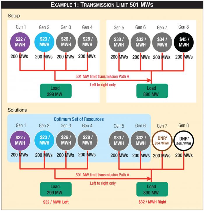 Example 1: Transmission Limit 501 MWs
In this case, the system would be considered uncongested, or unconstrained. Market prices are uniform across the system except for an adjustment for losses, which we are ignoring. However, if the transmission system is not capable of delivering all energy under optimum dispatch, the system is deemed to be congested or constrained, and prices diverge on each side of a congested line. Uncongested systems are rare, but a good place to begin the examples.
Example 1: An Unconstrained System Results in Uniform Prices
Assumptions: For the simplest of our examples, we will assume 501 megawatts of transfer capability on Path A and assume that loads and offers are as described in the graphic.
To determine the day-ahead price, the ISO performs the following process:
Determine Total System Load: The total load to be served is the sum of 299 megawatts in the Left Region and 890 megawatts in the Right Region, which is 1,189 megawatts.
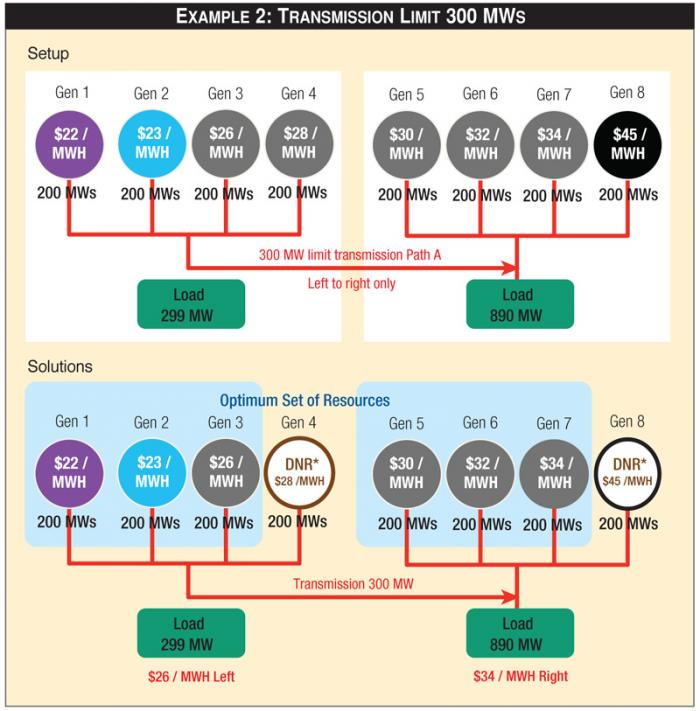 Example 2: Transmission Limit 300 MWs
See Example 1 Setup.
Determine the optimum set of resources or least-cost offers to meet total system load: The ISO will start with the unit with the lowest offer price, Gen 1, and continue in order of lowest price through Gen 6, until the load of 1,189 megawatts is met. To determine the market price based on marginal costs, the ISO asks what the cost would be to serve one additional megawatt. Because Gen 6 is needed at a dispatch level of 189 megawatts of its 200 megawatts offer volume, there is additional capacity available for this unit, so Gen 6 is designated as the marginal unit which will set price.
Determine if the optimum set of resources is feasible by testing the transmission limit. The generation selected in the Left Region is a total of 800 megawatts; that is, the sum of supply available from Gen 1 through Gen 4. 299 of the 800 will flow to serve load within the Left Region, leaving 501 megawatts to flow across Path A. Since Path A has the capability to flow 501 megawatts, the entire optimum set of resources is feasible, and this is the set that will be selected by the ISO to run.
Determine prices: When the optimum set of resources is feasible, energy prices are equal to the offer price of the marginal unit for all locations on the grid. In this case, the marginal unit is Gen 6 with an offer price of thirty-two dollars per megawatt-hour. Prices are set at thirty-two dollars per megawatt-hour for both regions. All generators scheduled will be paid thirty-two dollars per megawatt-hour and all loads scheduled will pay thirty-two dollars per megawatt-hour. Gen 7 and Gen 8 will receive no revenue, since they are not scheduled.
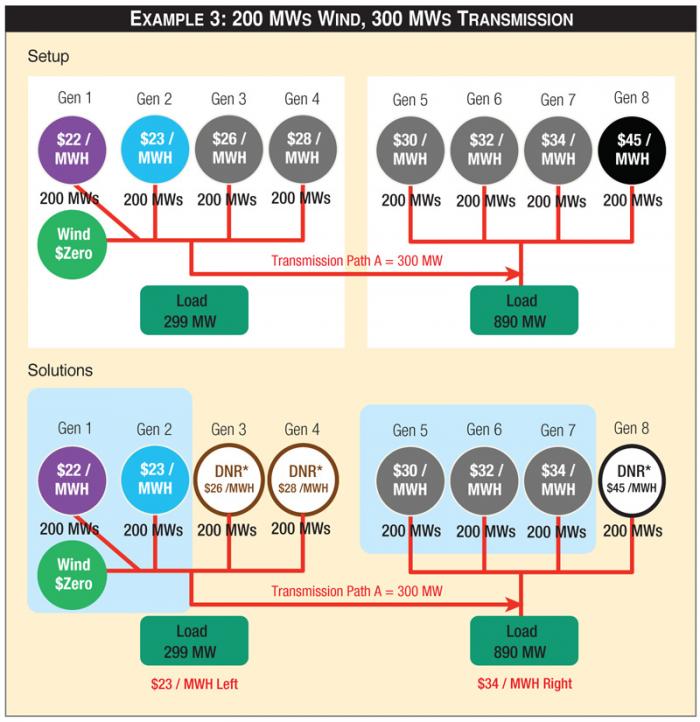 Example 3: 200 MWs Wind, 300 MWs Transmission
Example 1 Conclusions:
ISO energy prices are a function of three variables: volume of load, generation offers including volumes and prices, and transmission typology. From the unconstrained example, we can observe that in the absence of transmission congestion, all generators on the system receive the same price and all loads pay the same price.
Note that even if generators have long-term fixed-price bilateral contracts, these are not relevant to the ISO in determining dispatch. All that is relevant to the ISO is the supply offer from the generator, which is usually close to or equal to the generator's variable cost of operation and the level of load bids.
Because dispatch is based on the most economic bucket of generation needed to serve total load, it is impossible to determine which units serve which loads. As the solution diagram indicates, even if the LSE owns a specific generator, it is not possible to say that the generator has served that specific load. Therefore, all loads pay the same price regardless of connections to a generator.
 Example 4: 600 MWs Wind, 300 MWs Transmission
See Example 1 Solutions.
Example 2: A Constrained System Creates Price Separation
Assumptions: To show the impacts of congestion on Path A, we will keep all offers and bids the same, but now change the capacity of Path A to 300 megawatts.
See Example 2 Setup.
Determine which units will run on the Left: Since the offers are lower in the Left Region than Right, the generation on the Left will be maximized. The maximum allowable generation is 599 megawatts (299 megawatts load plus 300 megawatts transmission). Therefore Gens 1 through 3 will run, but unlike the previous example, Gen 4 will not be scheduled.
 Example 5: 600 MWs Wind, 700 MWs Transmission
Determine prices for the Left Region: The marginal unit from the Left Region (Gen 3) sets the prices for the Left Region at twenty-six dollars per megwatt-hour for both Left load and Gens 1 through 3.
Determine which units will run on the Right: The Right Region is receiving 300 megawatts from the Left Region via the transmission system. Therefore, it only needs to produce 590 megawatts on its own. (890 megawatts of load, less 300 megawatts from the Left). Gens 5 through 7 (Gen 7 at 190 megawatts) will run.
Determine prices for the Right Region: The marginal unit from the Right Region (Gen 7) sets the prices for the Right Region at thirty-four dollars per megwatt-hour for both Right Load and Generators 5 through 7.
See Example 2 Solutions.
Comparing Constrained and Unconstrained Results
We can now make further conclusions about the behavior of ISO markets. By comparing the price differences between Example 2 and Example 1, the impact of congestion can be determined. Congestion results in increased revenues for some generators and decreased revenues for others.
A similar impact occurs for loads, reducing costs in one region and increasing costs in another. For market participants, the change can mean many millions of dollars a year.
Comparisons can also be used to determine impacts of a transmission project, expanding Path A from 300 megawatts to 501 megawatts. If transmission were expanded, generators in the Left Region would see revenues increase, while generators in the Right Region would see revenues decrease. But loads in the Right Region would benefit, while loads in the Left Region would see their costs increase.
In many ISOs, all loads share part of the transmission expense. The load zones experiencing an energy price increase may be expected to pay tens of millions of dollars toward transmission expansion projects that result in millions of dollars of increased energy costs to them.
The next example adds 200 megawatts of wind generation in the Left Region. In each of the remaining examples we use the processes developed in Example 2 to determine which units run and the prices in each region.
Example 3 Assumptions:
A 200-megawatt wind project is added in the Left Region and the unit offers its energy to the ISO at a zero price. The 300-megwatt transmission limit and all other offers and bids are kept the same as in the prior example.
See Example 3 Setup.
See Example 3 Solution.
Comparing Before and After Adding Renewables
Here we see renewables displace coal generation (Gen 3). The addition of renewables also significantly decreases energy prices in the Left Region. In this case, the Left Region saw price decreases disadvantaging generation, but advantaging loads in the region.
Meanwhile in the Right Zone, there is no price impact. Interestingly, if the sponsor of the wind project serves load in the Right Zone, the sponsor paid to build a project that provides price benefits to someone else (loads in the Left Zone). And if that sponsor also owned Gen 3, they will see their generation revenue decrease from $26 to $23.
This demonstrates the critical need to study transmission typology and model market outcomes before assuming how historic energy price behavior will change with the introduction of new projects.
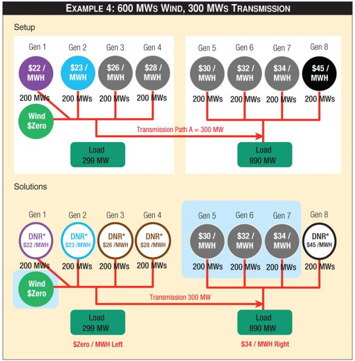
Example 4: Additional Renewables Displace Nuclear or Gas Units
Next, we'll see how adding additional renewables may not have the desired effect of reducing greenhouse gas emissions. Depending on transmission capabilities, adding more renewables may result in displacing nuclear or gas units while coal units continue to run.
Example 4 Assumptions:
The wind project in the Left Region is expanded by 400 megawatts, making total wind generation of 600 megawatts. All other assumptions remain the same.
See Example 4 Setup.
See Example 4 Solution.
Comparing Before and After Adding More Renewables
Here, we can see that the introduction of new renewables may not impact generation emissions as expected. In this case, the new wind capacity in the Left Region displaces nuclear and gas units while the coal units in the Right Region continue to run.
In this case, there is insufficient transmission capacity to move the "clean" power to loads. Meanwhile, generators located within the same zone as the renewables see sudden and significant revenue losses. In an extreme case, that could result in nuclear units and gas units being taken out of service while coal units on the other side of the constraint continue running.
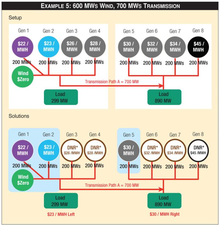
Example 5: Additional Transmission
Last, we'll see that transmission capability can be effective in reducing greenhouse gas emissions given the right conditions.
Example 5 Assumptions:
Path A adds 400 megawatts of transfer capability between regions, resulting in a total of 700 megawatts of transfer capability. All other assumptions remain the same as the previous example.
See Example 5 Setup.
See Example 5 Solution.
Comparing Before and After Adding Transmission
Here we see that under the right conditions, transmission expansion can be more effective in reducing emissions than building more renewable generation. But of course, market participants in the different regions see a side effect of increased or decreased economic results.
Actions by policy makers to achieve one goal, in this case to reduce emissions by building transmission, resulted in benefits for generators in the Left Region and disadvantages for generators in the Right Region. Similarly, loads in the Left Region had a disadvantage while loads in the Right Region got the benefit of lower supply costs.
Understand the Impacts of Actions
You now have deeper insight into how adding low-cost generation or generation with price supports allows certain units to offer lower prices into the ISO. And how decisions to expand, or not expand, transmission paths can have huge financial impacts on existing generators and loads.
Loads subject to capacity payments or generation subsidies may have to pay additional costs in these markets, and then discover that their energy costs also went up due to energy market outcomes. Similarly, market participants asked to pay for transmission expansion may not receive the benefits of the expansion and in some cases, may be disadvantaged through energy markets. And, the addition of low-carbon generation sources may not have the desired overall impact on emissions.
We suggest that all market participants, regulators, and policy makers start with the basic principles demonstrated here to begin developing an understanding of the interplay between new generation, generation subsidies, transmission expansion, and market outcomes.
And once you go beyond two regions, the analysis becomes much more complex, and sophisticated modeling must be used.
As FERC and various states consider different forms of price support for favored generation types and/or consider new transmission projects to foster generation development, it is important to realize that potential impacts may go well beyond the cost of subsidies paid to generators or the cost of expanding transmission.
In addition, the results of the energy market will benefit some market participants and penalize others. We contend that it is critical for regulators, policy makers, and renewable investors to thoroughly evaluate such impacts before choosing a course of action.
