
Charles D. Feinstein is an associate professor of operations management and information systems at Santa Clara University and the CEO of VMN Group, LLC. Jonathan A. Lesser is the president of Continental Economics, Inc.
Appendix:
Mathematical Structure of the Methodology
In this appendix to “Opening the Black Box,” (Fortnightly, January 2014), we briefly describe the basic components of the models for managing aging assets: how to represent the condition of such assets and the outcome of replacement, maintenance, and testing decisions.
The model structure is one of optimal control with dynamic state variables and uncertainty. Let
 = asset population that is in state s at time k.
The subscript indexes chronological time, measured in years, during the analysis period, which is can be represented as the interval  , for some arbitrary number of years, Tf , called the planning horizon.
Generally, there are three important aspects of the formulation of asset state dynamics. First, the distribution of the asset population among the states in the next year is a function of the current distribution. For instance, in the simple case that the state is the asset’s service age, and assets do not fail, the population at service age t in year k equals the population at service age t+1 in year k+1
 .
.
Second, the migration of assets among the states occurs probabilistically. Again, for simplicity, let the state s be the age t. If assets fail at age t at the rate h(t), then the surviving population of age t+1 in year k+1 is
The function h(t) is the hazard rate for assets. The hazard rate is determined empirically, using some generally applied functional forms, such as a piecewise linear or a Weibull nonlinear hazard function. In general, the members of the surviving population in any year migrate from state to state according to a collection of state transition probabilities. For example, it is simplest to think of annual changes in state, such that a transformer known to be in good condition at the beginning of a given year can be in either good, fair, or poor condition at the end of the year. Three transition probabilities determine the relative likelihood of these transitions: pgoodgood, pgoodfair, and pgoodpoor. These probabilities sum to 1.
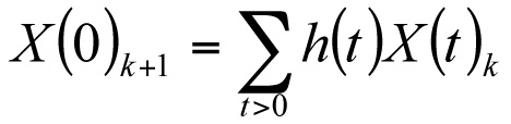
Third, the migration of assets among the states can depend on some action taken with respect to a particular asset in a particular state. For instance assets that are to be replaced as a consequence of the state-dependent optimal policy or that have failed may be replaced with new assets, so that the population of new (that is, age 0) assets at the beginning of the next year is the total of the assets of all ages that are replaced in the current period.
The condition of an asset can be tested, but all tests are imperfect. Hence, the consequence of the test is to revise the probability distributions on the asset condition. We write the likelihood that the test concludes that the asset is in condition cl when the actual condition of the assets is cj as the probability p {”ci”| cj}. (The quotations around the condition cl suggest that the test is making a claim that need not be true.)
As a result of the test outcome, the probability distribution on condition is revised. This revision is accomplished by application of Bayes’ Theorem, which determines the (posterior) probability that the assets is in state cj given that the test says that it is in any state cl:
 .
.
This equation, valid for all states {cj} and all ages t and all times k, permits the hazard rate to be updated as a result of the test. Therefore, the test-outcome-based hazard rate can be found:
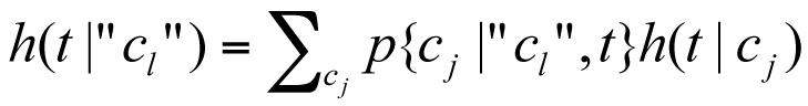
where h(t|cj) is the conditional hazard rate for an asset of age t in condition cj.
Minimization of Expected Costs
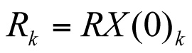
The costs associated with the asset inventory are the replacement cost, the failure cost, the cost of testing, the maintenance (or overhaul) cost, and operating costs that are associated with the unobservable states. In general, such a cost is based on the probability of the asset occupying any of the unobservable conditions. Let R = the cost of replacing an asset. Then the cost of replacements in year k is
Let F = the cost of an asset failure. Let (t, f) be the age and condition of any asset. Then the total cost of failures in year k is
 .
.
Let τ = the cost of testing an asset. Then the cost of testing in year k is
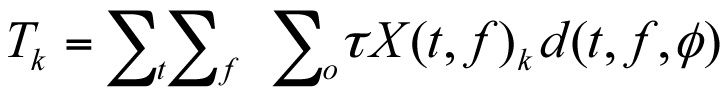
where the third argument in the decision function, d(t, f,”c”), which is the test outcome, is null and the summation is over all states (t,f) such that the value of the decision function 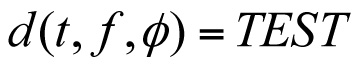 .
.
Let V = the cost of maintenance or repair. Maintenance or repair can be chosen before or after a test is done. There are two terms in the cost of maintenance or repair. Then the cost of maintenance or repair in year k is

where the summations are over all pairs (t,f) such that 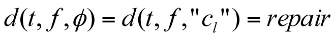 .
.
Let  = the operating cost of a asset if it is in (unobservable) condition cj. Then the operating cost in year k is

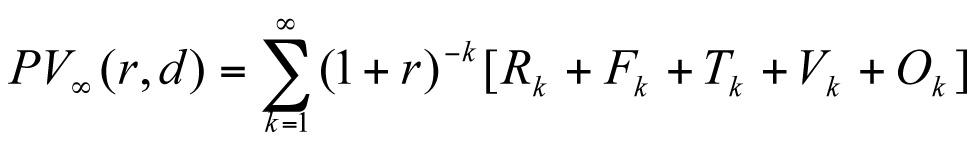
where the probability distribution on the unobservable condition is modified by the test outcome if testing were chosen. Then, the present worth of the policy that makes decisions d(t, f,”c”) is, for annual interest rate r:
 .
.
The decision problem is to choose the decision rule d(t, f,”c”) that minimizes the present value of the policy. The solution to this optimal control problem is the optimal policy for managing aging assets.
