
ERCOT load growth: patterns, possibilities, and second thoughts.
Ken Monts is a senior planning analyst at ERCOT, the Electric Reliability Council of Texas.
Through August 31, ERCOT's 2013 system load was 223 TWh (223 million MWh). Had ERCOT's 2013 capital stock retained its 2010 characteristics for energy intensity - i.e., energy use per unit of economic activity - the system load by that same date would likely have hit 237 TWh, or 6.3% higher than actual.

For the prior year, 2012, ERCOT's annual load (Jan-Dec) was 327 TWh. Again, however, if ERCOT's 2012 capital stock for electricity end uses (e.g., residential and commercial lighting, residential and commercial space conditioning equipment, industrial process equipment, etc.) had retained its 2010 energy intensity, then 2012 load would likely have reached 339 TWh - 12 TWh higher than actual.
Controlling variables and projecting energy intensity patterns forward can be instructive. For example, let's make several initial assumptions in an effort to predict total ERCOT annual system load for 2024, ten years out. First, assume that 2012 weather patterns prevail unchangingly every year throughout the 2014-24 interval (i.e., the dry bulb temperature at 4 a.m., July 17, 2019 is the same as the DBT at 4 a.m., July 17, 2012). Second, we also assume the Base Case forecast of Non-Farm Payroll Employment for each Texas county that Moody's provided to ERCOT staff in November, 2013. Third, we assume that ERCOT's capital stock is "frozen" and retains its 2013 (not 2010) energy intensity throughout the entire period, 2014-2024. On this basis, we can reasonably expect ERCOT's 2024 annual system load will be around 403 TWh.
But if assumption #3 will not hold, and if instead we expect that ERCOT's capital stock energy intensity will change over the 2014-24 interval in the same manner as it we have seen it change during the 2010-13 time period - i.e., if we assume that the same compound annual growth rate (CAGR) in energy intensity for 2014-24 as for 2010-13 (in this case, a decline) - then we might expect the 2024 system load to reach only 358 TWh, or fully 45 TWh less than what it would have been with the 2013 efficiency level still frozen in place.
As will be examined throughout this report, the recent changes in ERCOT utilization patterns have been dramatic. Should they continue, then future ERCOT system load surely will exhibit a significant diminution.
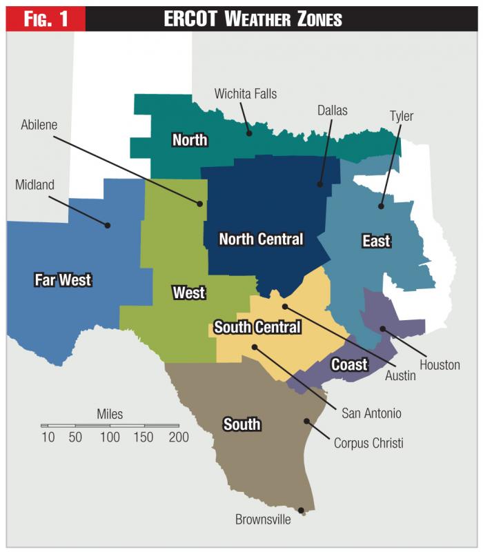 Figure 1 - ERCOT Weather Zones
And so we reach a looming question: are recent trends "the new normal" or, rather, are they unique and unlikely to be sustained?
This report will describe ERCOT's historical energy intensity patterns for 2010-13 (both graphically and mathematically) and then, in a highly preliminary fashion, will explore future possibilities by taking current measures of energy intensity (both as they are trending now, and by contrast, if they should become "frozen" over time), and then comparing those measures against the national energy intensity forecasts provided by the U.S. Energy Information Administration in its 2013 Annual Energy Outlook (AEO).
Before we get started, let's look ahead briefly with an example to illustrate what we're about. If we assume that the energy intensity patterns of the AEO's Reference Case hold for ERCOT over the 2014-24 interval, then we might expect ERCOT's 2024 annual system load will be 389 TWh - for a 2014-24 compound annual growth rate of 1.38%. That would be EIA's prediction. And as we can see, that CAGR would be considerably lower than the CAGR implied by our 2013 Frozen Efficiency case, but also considerably higher than our 2010-13 Current Trends case. Hence, from this comparison, we might infer that EIA does NOT expect ERCOT's recent energy intensity trends (2010-13) to prevail long-term for the nation.
Regional Energy Intensity
In the past, a particularly useful construct for examining energy demand patterns has been the concept of energy intensity. Energy intensity is always expressed as a ratio of two quantities: (1) some measure of energy (kWh, joules, barrels-of-oil-equivalent, tons of coal, cubic feet of natural gas, British thermal units, etc.), divided by (2) some other quantity (number of people, number of households, $GDP, number of commercial building square feet, number of non-farm payroll jobs, etc.). Energy intensity indicators are particularly useful for examining energy efficiency trends. Caution must be exercised , however. Many factors can affect energy intensity - even apart from such things as the saturation of energy-efficient appliances. For example, if an aluminum smelter or a large data center locates in a smallish area, then that area's aggregate energy intensity will likely increase, even if every residence is retrofitted with 18 SEER air conditioners. Nonetheless, over large areas like ERCOT's weather zones (see Figure 1), energy intensity indicators will likely provide strong clues regarding matters such as energy efficiency.
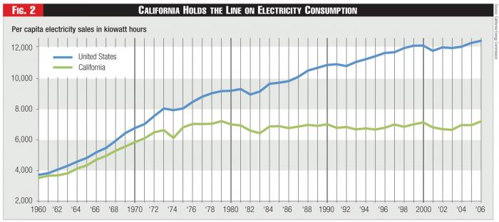 Figure 2 - California Holds the Line on Electricity Consumption
Annual kWh-per-capita is probably the most straightforward energy intensity indicator and is often used in an attempt to capture energy efficiency trends. Probably the most notable study of this simple indicator is the oft-mentioned Rosenfeld curve (see Fig. 2), named after Arthur Rosenfeld, a former member of the California Energy Commission. The Rosenfeld curve1 depicts the stark contrast since the early 1970s between California's per-capita electricity consumption (in kWh) versus the rest of the nation. Other indicators beyond kWh-per-capita are useful as well. An earlier EIA document2 provides a particularly lucid discussion of the construction and interpretation of energy intensity indicators, generally.
This report will focus heavily on a single, particular indicator of energy intensity, known as DEPJ, or daily energy (in MWh) per number of jobs, as measured in the 1000s. Under this measure, daily energy is the daily MWh for a specific day for a specific ERCOT weather zone3 and is derived by summing the 24 hourly values for each day 2010-13. The term "Jobs" refers to Non-Farm Payroll Employment,4 as reported monthly by the U.S. Bureau of Labor Statistics monthly-reported and (in this case) as aggregated up to the weather zone by summing across all the counties in each weather zone.
Figure 3 graphically displays a single instance of the central analytical finding of this report. This figure represents all August weekdays (2011-13) for the South Central ERCOT weather zone (which includes San Antonio and Austin). Please note several features.
First, DEPJ is highly correlated with Average Daily Dry Bulb Temperature (r-squared=0.944), when year is included in the model specification (and with ADDBT measured as Maximum Daily Dry Bulb Temperature plus the Minimum Daily Dry Bulb Temperature, divided by two). Second, the relationship is linear (for summer months) with a slope that indicates that DEPJ increases 1.8399 dailyMWh/nonfarm-job for every one degree increase in Average Daily Dry Bulb Temperature. (By contrast, the relationship is quadratic for winter and spring/fall months). Third, however, and most significant, while the slope appears to be strikingly constant across the 2011-13 years, the intercept with the y-axis is significantly different for each of the three years. Thus, the year 2011 intercepts the y-axis at a point considerably greater than does 2013, while the 2012 intercept rests in between 2011 and 2013. In other words, daily electricity consumption per nonfarm job was falling during this period in ERCOT's SouthCentral Weather Zone.
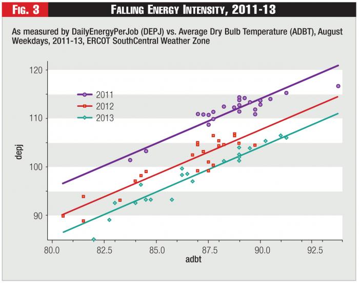 Figure 3 - Falling Energy Intensity, 2011-13
Such results as suggested by Figure 3 lend themselves readily to a particular statistical technique known as Dummy Variable Regression Analysis.5 Figure 4 displays the output from applying the SAS procedure known as PROC GLM©6 to the data in Figure 3. The most significant features, for our purposes, are the coefficients of the three years captured by the "year" dummy variable. A straightforward interpretation is that the year 2011 adds 9.91159 dailyMWh/nonfarm-job to the intercept and the year 2012 adds 3.4961 dailyMWh/nonfarm-job, while the same slope (1.839972) holds across all years. This same pattern can be seen in dramatic fashion in six of the other seven ERCOT weather zones. The only exception is the Far West, where the year 2013 is the most energy intense - presumably because of so much energy development activity seen in that region of late.
These results from Figure 4 suggest several interesting lines of exploration. First, backcast what the 2010-13 load would have been if the change had not occurred. (The results of that exercise were reported in the opening section of this report). Second, derive a compound average growth/decline rate from the trend suggested by the year dummy coefficients, extrapolate those growth/decline rates into the future, and examine what ERCOT's load would be if those rates remained the same throughout the 2014-24 time period. For example, by using the 2010-13 data (only 2011-2013 was used in the graph for illustrative purposes, but the same results obtain when 2010 is included) CAGR calculations were carried out for all eight ERCOT weather zones and the results were used to construct a "Current Trends" scenario. As noted above, this analysis produced a 49-TWh diminution in projected 2024 load. Third, one might compare the Current Trends and the Frozen Efficiency 2013 scenarios with a set of alternative energy intensity scenarios derived from the Energy Information Administration's 2013 Annual Energy Outlook.
Figure 5 displays 2014-24 annual loads corresponding to the Frozen Efficiency 2013 scenario and the Current Trends 2010-13 scenario. As earlier stated, the aggregate effect of projecting the 2010-13 energy intensity changes to continue at the same rate throughout the 2014-24 interval has significant impacts. Despite relatively robust economic growth, the ERCOT system load increases only to 358 TWh by year 2024. Whereas, the Frozen Efficiency scenario displays robust load growth in tandem with economic growth. Clearly, our initial underlying assumptions regarding the future growth (or decline) of energy intensity will have considerable significance in any attempt to project future load levels.
Nationwide Scenarios
Now let's turn to nationwide trends, as observed by the U.S. Energy Information Administration.
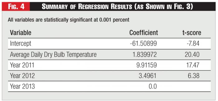 Figure 4 - Summary of Regression Results (as Shown in Fig. 3)
In its Annual Energy Outlook, the U.S EIA presents "...long-term projections of energy supply, demand, and prices through 2035 based on results from EIA's National Energy Modeling System (NEMS)." 7 The energy demand module of NEMS comprises a detailed end-use representation of residential, commercial, and industrial sectors. The residential sector alone represents 24 end-uses for three different housing types.8 A primary use of NEMS is to accommodate requests related to scenario analysis, such as from the U.S. Congress, and others.
In its AEO 2014, Table E1,9 the EIA presents a concise description of the 26 predefined scenarios explored in the 2013 Annual Energy Outlook. Most significant for our purposes are (1) the Reference Case, (2) the Integrated High Demand Technology Case, and (3) the Integrated Best Available Demand Technology Case.
A comprehensive description of these scenarios can be found in the 2013 EIA Annual Energy Outlook. In particular, AEO 2013 depicts a nice curve (Figure 52, p. 59) that shows historic energy-use-per-capita as far back as 1980, and projected forward to 2040, illustrating a slight downward trend. Of this downward trend in energy use per capita (much less severe than the drop over the same period in energy use per dollar of GDP), the EIA notes as follows:
The decline in energy use per capita is brought about largely by gains in appliance efficiency and an increase in vehicle efficiency by 2025. From 1970 through 2008, energy use dipped below 320 million Btu per person for only a few years in the early 1980s. In 2011, energy use per capita was about 312 million Btu. In the Reference case, it declines to less than 270 million Btu per person in 2034 - a level not seen since 1963.10
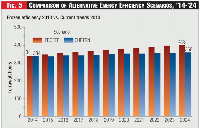 Figure 5 - Comparison of Alternative Energy Efficiency Scenarios, ’14-’24
Note that the most precipitous decline in the slope depicted in EIA's Figure 52 (for energy use per capita) occurs after 2025. By comparison, the 2014-24 time period shows a much gentler decline. The implication is that the EIA Reference Case expects the national energy intensity to start its decline at a very gradual rate in the first ten years. Not so, however, for the other two EIA Technology cases considered here: (1) the High Demand Technology Case, and (2) the Best Available Demand Technology Case. Here is what EIA says in AEO 2013:
The High Demand Technology case assumes higher efficiency, earlier availability, lower cost, and more frequent energy-efficient purchases for some equipment. The Best Available Demand Technology case limits customer purchases of new and replacement equipment to the most efficient models available at the time of purchase - regardless of cost. This case also assumes that new homes are constructed to the most energy-efficient specifications.
From 2011 to 2040, household energy intensity declines by 31 percent in the High Demand Technology case and by 42 percent in the Best Available Demand Technology case.11
Each of these three scenarios was examined here and a preliminary implementation was prepared to depict future ERCOT load possibilities based on these EIA-projected scenarios to compare with the Frozen Efficiency 2013 and the Current Trends 2010-13 scenarios that are specific to the ERCOT region.
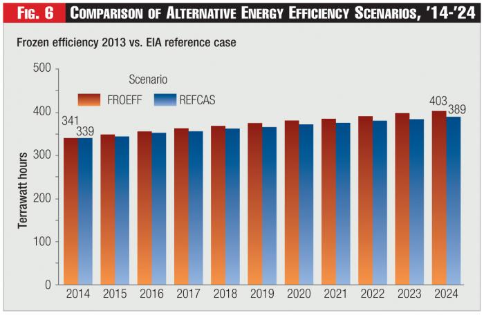 Figure 6 - Comparison of Alternative Energy Efficiency Scenarios, ’14-’24
The next step was to construct energy intensity growth/decline rates for the scenarios defined by the EIA, and for specific energy uses. In our case, this step was accomplished by extracting information from the detailed statistics prepared by EIA for each scenario and available using web links to certain EIA data collections.
Consider three different types of residential energy end uses: (1) Residential Space Cooling, (2) Residential Space Heating, and (3) Residential Base Load - reflecting most other uses, such as refrigeration, cooking, clothes washers, dish washers, televisions, computers, other uses.) A link12 to the Reference case at the Annual Energy Outlook 2014 Early Release provides access to data that can be used to connect the several EIA scenarios with these specific energy uses.
For example, the Early Release presents the number of households in year 2013 (114.39 million) all the way through 2040, with 135.91 million assumed in year 2033. The same report details the energy use for each end-use. From these data, Residential Space Cooling national energy use in 2013 is assumed to be 0.70 quadrillion Btu growing to 1.12 quads in year 2033. Dividing 0.70 quads by 114.39 million households produces the national space cooling energy intensity in 2013 (virtually all of it electricity). Next, for space cooling, dividing 1.12 quads by 135.91 households in 2033 yields the space cooling energy intensity that EIA's end-use modeling system forecasts for the nation for their Reference case. From that, a 20-year compound annual growth (decline) rate can be calculated. The same calculations can be done for space heating. A third growth rate can be calculated for the base loads (primarily plug loads) noted above, but a little more involved to derive a compound growth rate for the aggregate group.
Finally, to allow for a meaningful comparison between data from EIA and ERCOT, the space cooling and baseload growth rates are combined and applied to all summer months (May-September) to implement the ERCOT-equivalent scenarios. The space heating and baseload rates are combined and applied to winter months (Dec-Jan-Feb). The baseload growth rate alone is applied to spring/fall months (Mar, Apr, Oct, Nov).
Doubts and Suspicions
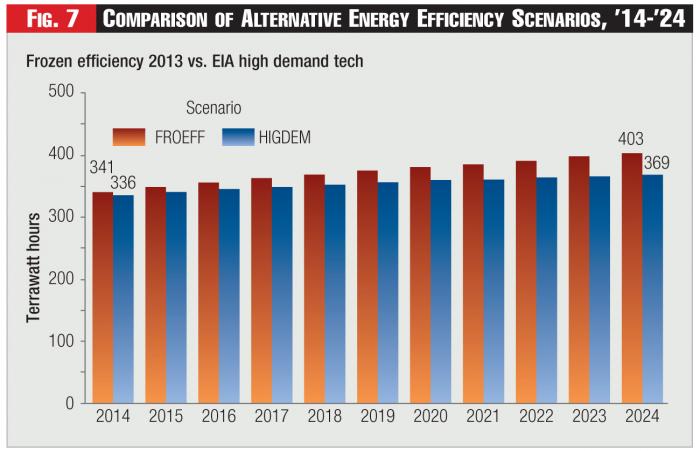 Figure 7 - Comparison of Alternative Energy Efficiency Scenarios, ’14-’24
The results of this implementation must be interpreted as highly tentative at best.
On one hand, the assumption is that growth/decline rates of one energy intensity indicator (Btu-per-household), for one specific sector (residential), for a broad geographic sector (U.S.) can be meaningfully applied to another energy intensity indicator (dailyMWh-per-job), for a different geographic entity (Texas), and applied across all sectors. In more colorful terms, we might as well ask, "As the nation goes, so should go Texas?" Some might justifiably beg to differ.
Still, as "heroic" as some of these assumptions appear, the fact of the matter is that year 2025 will eventually roll around. By that date, there WILL have occurred, willy-nilly, an energy intensity growth rate in the 2014-24 interval - whether it be kWh-per-capita or dailyMWh-per-job. That is to say, at that point, it will be an inexorable fact. Furthermore, mathematics will still be around and we WILL be able to calculate what that rate actually was. In 2014, however, we can only guess what it might be. Given its importance, it probably behooves us to try to leverage as much constructively useful information as possible to inform that guess, just as we want to try to inform our guess of future economic and population growth and our guess as to what is the likelihood of a reoccurrence of 2011 weather.
Figure 6 displays a comparison between the Frozen Efficiency scenario and the EIA Reference Case. As previously mentioned, the EIA Reference Case culminates in a 2024 ERCOT load of 389 TWh - significantly lower (i.e., greater efficiency and less intensity) that the Frozen Efficiency 2024 load of 403 TWh but significantly higher (less efficiency, more intensity) than the Current Trends scenario.
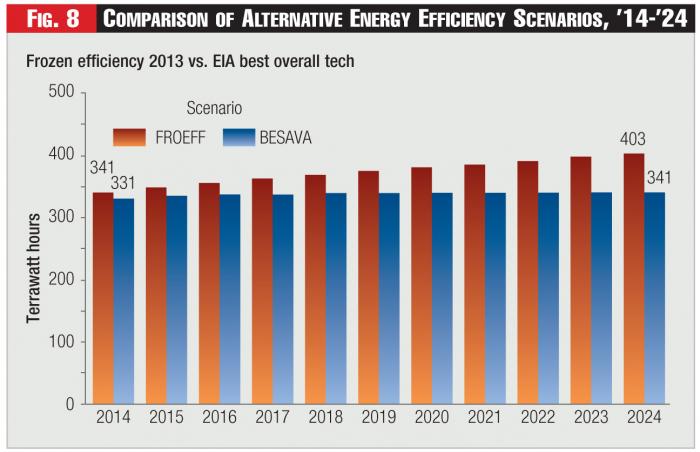 Figure 8 - Comparison of Alternative Energy Efficiency Scenarios, ’14-’24
Figure 7 displays a comparison between the Frozen Efficiency scenario and the EIA High Demand Technology scenario - which yields a 2024 load of 369 TWh. As expected, this scenario is significantly below (more efficient, less intensive) both the Frozen Efficiency scenario and the EIA Reference Case.

Figure 8 displays a comparison between the Frozen Efficiency scenario and the EIA Best Available Technology scenario - which yields a 2024 ERCOT system load of 341 TWh.
What is most striking about these figures is that of the EIA scenarios, only the Best Available Technology scenario is lower (more efficient, less intensive) than the ERCOT Current Trends scenario - but even then, not by all that much. And remember: the Best Available Technology (BAT) scenario is essentially a "science fiction" construction that the EIA set up for comparison purposes and not something to be taken seriously as something that could actually occur. It essentially posits that every new house constructed between 2014 and 2024 will have an air conditioner with a Seasonal Energy Efficiency Ratio of 18 plus - and R30 wall insulation. Every square foot of commercial buildings constructed will have some form of advanced variable-air-volume HVAC with advanced electronic controls. And, so forth.
Thus, with the ERCOT Current Trends scenario appearing not all that far off from the EIA's essentially fictional BAT scenario - achieving similar reductions in energy intensity - the ERCOT Current Trends scenario would seem to be suspect. These results are suggestive that SOMETHING has been happening to ERCOT's capital stock in the last few years that tilted the energy intensity growth (decline) rates, and, furthermore, that a projection of those rates forward should be approached with some trepidation.
We can only speculate what that SOMETHING was. However, it seems likely that a major factor has been the truly historic level of public investment in ERCOT's energy-using capital stock. For example, the U.S. DOE awarded, as part of the State Energy Program, $75 million to the Building Efficiency and Retrofit Program, $76.8 million to the Distributed Renewable Energy Technology Program, $10 million to the ENERGY STAR Appliance Rebate Program, and $25 million to the Texas Cool School Program.13 The ARRA (American Recovery and Reinvestment Act of 2009) awarded $45 million to the Texas State Energy Conservation Office under the Energy Efficiency and Conservation Block Grant Program to be distributed directly to cities under 35,000 and counties under 200,000.14 The Energy Efficient Appliance Rebate Program was allocated $23 million.15
At the same time that these extraordinary levels of funding were occurring, the state-mandated expenditures as part of the Energy Efficiency Implementation Plan, Substantive Rule 25.181 and 25.183 were occurring at unprecedented levels. The ONCOR Electric Delivery Company reported a 2013 budget of $25 million for the Commercial sector spread across seven separate programs, plus $21 million for the Residential sector, and $13 million for the Hard-to-Reach customer, for a total budget of $62 million for the year 2013.16 That was on top of a budget of $49 million in the year 2012.17 CenterPoint Energy reported a 2013 budget for Large Commercial of $18 million, for Residential and Small Commercial $12 million and a total 2013 budget of $38 million.18 That was on top of their 2012 expenditures, which came on top of $26 million in 2011, $25 million in 2010, and $22 million in 2009.19
The years 2009, 2010, and 2011 are significant because that is what is being captured by the year dummy variables in our regression analysis of 2010-13 growth trends - an air conditioner retrofitted as a result of 2009 expenditures is still saving energy in 2010, 2011, 2012, and 2013. The effects are cumulative and savings attributable to 2013 investments are added to those brought about by 2009 investments - and the dummy variables capture cumulative effects.
Most likely, this level of public investment (federal and state) in a specific infrastructure (buildings) in a specific region (Texas) has not likely occurred at any time since the New Deal. Hence, perhaps the exceptional decline rates uncovered by the statistical analysis should not be viewed so much as a mystery. Perhaps, the 2024 energy projection resulting from their application makes sense. The only mystery might be whether we should take them seriously as any guide whatsoever for viewing possible ERCOT system load futures. Sometimes the future does not resemble the past and prudent planning would be well-advised to recognize potential departures.
New or Still Normal?
Hippocrates tells us, "Declare the past, diagnose the present, foretell the future."
That we live in uncertain times is a platitude. But regarding future electricity loads, an emerging consensus seems to be building that a "new normal" has been established. In their compelling analysis and description, Faruqui and Schultz convincingly posit:
When all is said and done, the drop in electricity demand seems to be permanent, not transitory. It would be a mistake to attribute this drop solely to the recession and assume it will go away once normal economic activity resumes.20
Still, even these confident authors provide some pause:
...some factors could drive demand growth higher in the coming years. The digitalization of life at home and in the workplace has increased the need for electricity to power new appliances and technologies. And plug-in electric vehicles, while saving customers substantial gasoline costs, will bring a major increase in electricity use. Also, increasing home size results in more energy consumption.21
Moreover, this ambiguity regarding the future of "poorly understood, amorphous" plug loads also causes chagrin for the authors of another excellent end-use study:
The basic assumption of the Low-Demand Baseline is that new technologies (both influencing cooling equipment and the building envelope) would keep pace with improvements in other technologies affecting other major end uses. The poorly understood, amorphous, and perpetually growing plug loads, usually termed "miscellaneous," are a concern for this approach and for buildings energy forecasting in general. If miscellaneous electricity intensity does not decline to the same degree as all other major building end-use intensities, then the future share of electricity associated with all other end uses - including cooling - will fall, but overall demand will NOT decline as projected.22
And a recent New York Times piece has trumpeted, "McMansions Are Making a Comeback":
In both 2008 and 2009, Census Bureau figures show, the median size of a new home was smaller than it had been the previous year. It seemed that after more than a decade of swelling domiciles, the McMansion era was over. But that conclusion may have been premature. In 2010, homes started growing again. By last year, the size of the median new single-family homes hit a record high of 2,306 square feet, surpassing the peak of 2007.23
No factor affects aggregate residential energy intensity to quite the extent as does the distribution of house sizes skewed either left or right. If there were to be sustained growth in new home house size, if "domiciles start swelling again," not only could the pace of change in energy intensity change, but, plausibly, even the direction of that change could shift, and ERCOT 2024 system load could easily go north of 404 TWh.24
These caveats aside, it would be difficult to review ERCOT's recent energy intensity patterns and find evidence supporting a resurging demand. Indeed, the recent trends have been so dramatic in the other direction that the main problem seems to be how does the analyst judge them in a judicious enough manner to be able to assess what the future may hold. To what extent has the recent prodigious public investment so distorted trends that extrapolation may pose significant risk to efforts to plan infrastructure and design markets? Sometimes diagnosing the present is not as straightforward as Hippocrates would like.
Endnotes:
1. See, Calif. Energy Comm'n, 2007 Integrated Energy Poicy Report (CEC-100-2007-008-CMF), Exec. Summary, p. 3.
2. See, U.S. EIA, Measuring Energy Efficiency in the U.S. Economy: A Beginning, Oct. 1995.
3. For availability of such data, see: http://www.ercot.com/gridinfo/load/
4. For a general definition, see: http://en.wikipedia.org/wiki/Nonfarm_payrolls
5. For a general explanation, see http://en.wikipedia.org/wiki/Dummy_variable_(statistics)
6. See, SAS Institute Inc.
7. See US EIA, "The National Energy Modeling System: An Overview," (DOE/BA-0581), Oct. 2009.
9. US EIA Annual Energy Outlook 2014, "NEMS Overview and Brief Description of Cases," Table E1. Summary of AEO 2013 Cases.
10. U.S. EIA, Annual Energy Outlook 2013, DOE/EIA-0383(2013) April 2013, Fig. 52, p. 59.
12. See, http://www.eia.gov/oiaf/aeo/tablebrowser/#release=AEO2014ER&subject=0-AEO2014ER&table=4-AEO2014ER®ion=0-0&cases=full2013-d102312a,ref2014er-d102413a
13. The State Energy Program provides federal grants that states use to promote energy conservation and efficiency, and to reduce energy demand.
14. http://www.seco.cpa.state.tx.us/arra/eecbg/index.php
15. http://www.seco.cpa.state.tx.us/arra/rebate/index.php
16. ONCOR Electric Delivery Co., LLC, 2013 Energy Efficiency Plan and Report, Project No. 41196, April 1, 2013, p. 36.
17. ONCOR Electric Delivery Co., LLC, 2012 Energy Efficiency Plan and Report, Project No. 40194, April 2, 2012, p. 19.
18. CenterPoint Energy Houston Electric, LLC, 2013 Energy Efficiency Plan and Report, Project No. 41196, April 1, 2013, p. 36.
19. CenterPoint Energy Houston Electric, LLC, 2012 Energy Efficiency Plan and Report, Project No. 40194, March 30, 2012, p. 40.
20. "Demand Growth and the New Normal," Public Utilities Fortnightly, December 2012, p. 22, at p. 28.
22. National Renewable Energy Laboratory, Renewable Electricity Futures Study, Vol. 3 of 4: End-Use Electricity Demand, NREL/TP-6A20-52409-3, at p. H-11.
23. McMansions Are making a Comeback, by Anna Bernasek, New York Times, published Nov. 23, 2013.
24. A recent study in Housing Economics, published by the National Asso. Of Home Builders, finds that the median size of new homes reached 2300 square feet in 2012, the highest figure since 1974, when data was first collected. See, "Characteristics of Homes Started in 2012: Size Increase Continues," by Paul Emrath, Ph.D., Aug. 1, 2013.
